Refining the process

So far, when I try to discriminate cloudy areas from usable data in a Landsat scene, I tell it to ignore everything that has a pixel value above 100 in band 3. This process discriminates a lot of unusable pixels that are clouds while avoiding the elimination of good pixels. This said, inspection of the band 5 histogram has inspired me to try to discriminate shadows in a similar way I use band 3 to get rid of clouds.

Histogram of band 5 of a close up of a Landsat scene

Close up of Landsat scene (pixels in red have a value inferior to 30)

As can be seen from the close up above and its histogram, discriminating pixels that have a value under 30 are almost exclusively cloud shadows. The exception being shadows that result of abrupt topography and water bodies.

Comparing an image where I discriminate only pixels that have a value above 100 in band 3 to an image where I discriminate both pixels that have a value above 100 in band 3 and pixels that have a value under 30 in band 5 gives the following results:

(If you ignore the stripes, green are pixels that should
be good data, yellow are pixels that have a value above
100 in band 3 [clouds] and red are pixels that have
a value under 30 in band 5 [cloud shadows, abrupt
topography shadows and water bodies])

Close-up of above scene

Further testing needs to be done to determine if I should use this thresholding method on band 5 and/or if the threshold value should be changed.

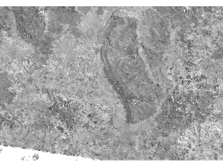
On a different note, I’ve observed that certain bands seem to be far better suited to the method I’m developing to create cloud free composites:

Close-up of Landsat cloud-free image
composite made from 12 images - Band 1

Close-up of Landsat cloud-free image
composite made from 12 images – Band 2

Close-up of Landsat cloud-free image
composite made from 12 images – Band 3

Close-up of Landsat cloud-free image
composite made from 12 images – Band 4

Close-up of Landsat cloud-free image
composite made from 12 images – Band 5

Close-up of Landsat cloud-free image
composite made from 12 images – Band 7

Close-up of Landsat cloud-free image
composite made from 12 images – Band 8

Unwanted artifacts far less impair band 4, 5 and 8 than the other bands.

Basic statistics for image composition

In an attempt to get rid of the pesky clouds that plague equatorial regions, namely Borneo, I’ve tested different approaches. For any given Landsat scene, I have access to images taken every couple of weeks. Now some of them are only slightly obscured by clouds.

Image least affected by cloud cover out of seven taken
over a period of four months (RGB composite)

False color composite of same image

Unfortunately, we’re usually not so lucky and it’s not unusual for a landsat scene taken over tropical regions to look more like this one.

Same scene as above…

Also, every Landsat scene taken since May 2003 have data gaps because of the SLC-off mode the satellite has been operating in.

The gaps and thick clouds are easily identified and removed, but filling those removed areas with data form other dates can prove challenging, as I shall illustrate.

For my first attempt, I used a cloud detection algorithm implemented as a GRASS add-on module : (i.landsat.acca.) I then combined the seven images I had at hand, minus their clouds and stripes, to create a new composite image.

Composite image made from seven images
with clouds removed with the i.landsat.acca
GRASS add-on module

As can be seen, there is a lot of data missing in the resulting image. As a matter of a fact, this image is more fragmented than the least cloudy image of the seven used to create the composite (see first and second image of this post.)

This led me to investigate how I could reassemble my seven images without using this module. I gave all the missing values (thick cloud obstruction and stripes) the value 255. None of the unsaturated pixel even comes close to nearing this value. I then crated a new image, pixel by pixel, using the minimum value for a given pixel out of the seven images. My premise was that the darkest pixel is the one least affected by haze or partial cloud obstruction (which makes the pixel pale; pale pixels have a higher value.) I obtained this resulting image:

Composite image obtained by using the minimal
value for each pixel out of seven images

The problem with this approach is that cloud shadows tend to be very dark. This explains the numerous dark patches, which can be seen in the image above. Unfortunately, when using the exact opposite approach, the resulting image includes lots of haze and outer edges of clouds:

Close-up of a composite image obtained
by using the maximal value for each
pixel out of seven images

What seems most promising is to use the median values of all the pixels that are neither clouds nor stripes. Because GRASS has trouble dealing with null values for pixel by pixel analysis, the images had to be exported into the statistical software R to extract the median values, than reimported into GRASS for further analysis.

Image composed of the median value
for each pixel (RGB composite)

Same image (false colors composite)

Close-up the same image (RGB composite)

Same close-up (false colors composite)

Now I need to see how useful this image can be to produce classifications or band ratios such as NDVIs.